
Apache Kafka is probably primarily known as a messaging middleware with a more flexible structure than queues, but it also empowers teams with its lower entry barrier for real-time data pipelines.
So-called stream applications using Kafka are scalable, are fault tolerant, and display strong ordering and delivery guarantees, besides having extensive integration for moving data in and out of Kafka clusters. Rather than having to carefully design, maintain, and test hand-rolled, data-intensive solutions, some applications can leverage Kafka Streams to do the heavy work.
But let’s not get ahead of ourselves. For the first of this two-part Snippets series, we’ll focus on basic stream processing operations in order to introduce some of the challenges involved. Basic knowledge of Kafka helps, but it’s not required; we’ll focus on a high-level view of streams and discuss how they are represented in Kafka only when necessary.
Basic Operations
First, the main abstraction in stream applications are, well, streams: a sequential and potentially unbound source of data. For instance, we could have a stream containing all the posts on a social network: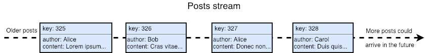
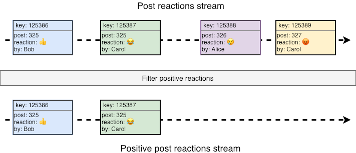
We can perform operations on streams. A simple one would be applying a filter to each record, producing another stream as a result. Suppose we have a stream of reactions to posts and we want to filter only the positive ones:
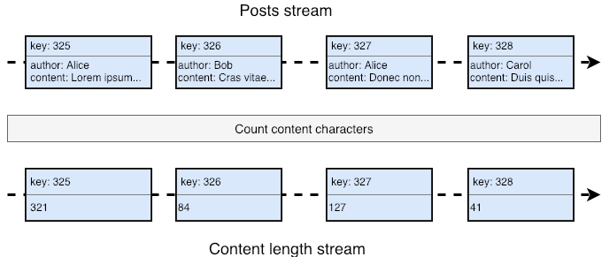
Another basic operation is transforming messages into a new output stream; in the following diagram, we are counting the characters inside each post to produce a stream of integers:
Quite intuitive, right? Time to move to something more complex. Instead of counting the characters inside a post, we are going to perform an aggregation: counting the number of posts by author.
Aggregations
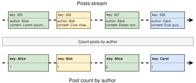
Notice that this aggregation updates and produces a new count every time a new post arrives. So instead of performing the aggregation every time we need this metric, as is usually done when using relational databases, a count in stream applications is a continuous reduction working only with the previous count and the record that has just arrived.
In Kafka Streams, the result of this aggregation is not actually a stream, but we’ll talk about that in a while. What is important right now is to notice that this is a stateful operation: to update the count once a new post arrives, we need the previous count by the same author. That's why it makes sense to change each record's key to the post's author, as shown in the previous diagram, allowing us to quickly get the previous count. Notice that since an author can take a long time to post something new, we'd need some sort of durable storage to persist each count. Keep this in mind, but let's move to another common stateful operation: joining streams.
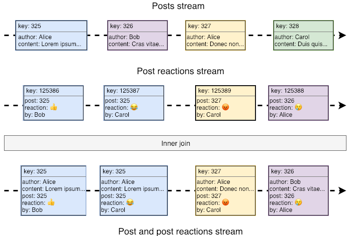
Suppose we need to find out whether post length and reaction are correlated. One way to start would be joining each reaction in the reaction's stream to its post. In a simple scenario, we’d have something like this:
This is a good starting point, but joining streams like this might not be possible. Remember, the stream is an unbound source of data, so there’s no telling when (or if) we’re going to get a new reaction to Alice’s post. To join both streams, we’d have to either keep posts around for an infinite amount of time, waiting for the next reaction, or, every time we get a reaction, we’d have to traverse the post stream looking for the post to join--which would hardly be called real-time stream processing.
Time Windows
Instead, in order to keep the data manageable, stream joins are performed within user-defined time windows.
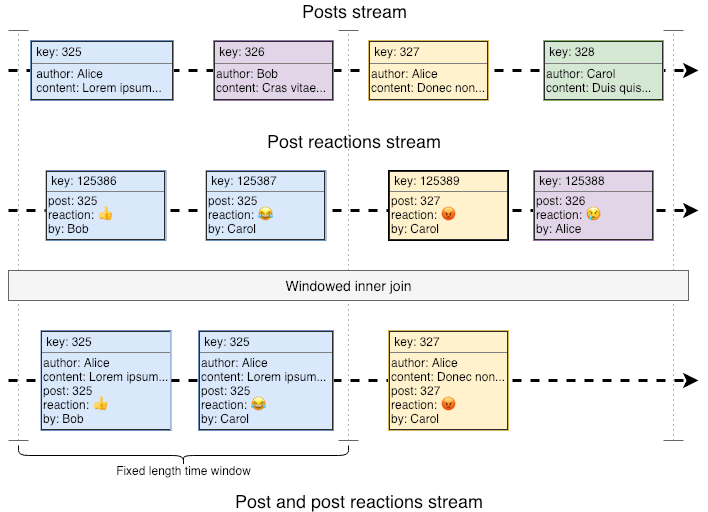
We perform the join only for posts and reactions that fall inside the same window, so metrics computed over this result would also be windowed (e.g. “based on the first 5 minutes after a post, we’ve seen that larger posts have X% fewer reactions”). Notice, however, that in this case, a bunch of future reactions that fall outside the time window will not be joined and so won’t be part of our metric. For instance, notice how Alice’s reaction to Bob’s post falls outside its time window. Actually, for anything computed on top of the join result, it would look like Bob’s post has no reactions at all. We could extend the time window, but that would only minimize the problem, not solve it.
What would be nice is if it was possible to perform a quick lookup by the post key for each incoming reaction in order to join the post and reaction without any time windows involved.
Tables
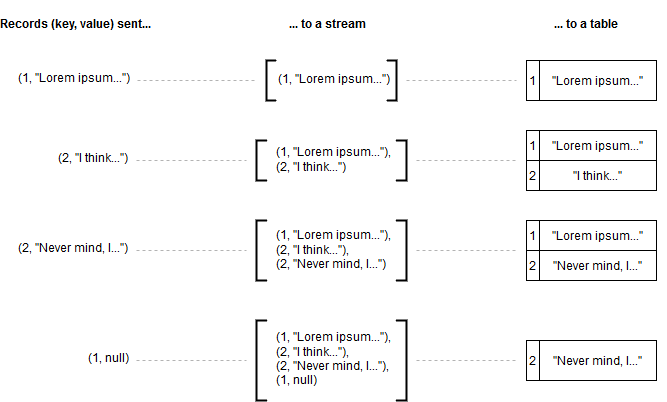
Enter tables. Tables are different data structures available in Kafka Streams. For a given key, they store only the last value seen, just like tables in relational databases. The image below shows the difference between storing records in streams and tables:
In Kafka Streams, the join semantics for streams and tables (in that order) are exactly what we need. Every time a new reaction arrives, Kafka will look up its post in the posts table and join the tuples. Under these semantics, joining reactions and posts would result in the following stream: 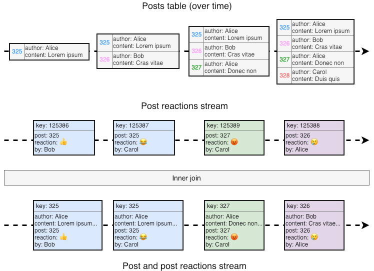
With this, we have an idea of what’s involved in stream processing: how streams work, the operations available, the complexity associated with stateful operations, and so on. That's great starting knowledge, but in preparation for the next part of this blog series, let's start going deeper.
How Streams are Represented
For instance, how are streams and tables represented inside Kafka? Well, it turns out that the same topics involved in plain Kafka are used to represent streams. If you're not familiar with them, you can think of topics as append-only lists, where each topic consumer keeps tabs of its position on the list:
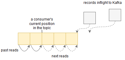
This naturally maps to a stream representation, right? New data is always inserted in the end of the topic, and consumers continuously read data from some point onward. Tables are also backed by topics, but they'll usually have log compaction enabled, meaning that for a given record key, Kafka might store only the last value received (which naturally won't be a problem for tables).
Keep in mind, however, that consumers are not limited to moving forward one position at a time. In fact, they have full control of their offset in a topic, being able to move back and forth however they see fit. This will be important when we talk about recovery in real-time stream processing applications! Besides discussing recovery in part two of this series, we’ll also cover other challenges involved in real-time stream processing, why they matter, and how Kafka solves them.
Until then, drop a comment if you have any questions or feedback. See you in the next snippet!


