Important note: this blog contains a brief summary of the developments of the Chicago Taxi Trips use case. For more details and information, please access the complete official document of this work.

This article shows a demo use case for Machine Learning prediction using an available dataset from Google Cloud containing all the Chicago Taxi trips from 2013 until 2018. The primary business need in this demo is to provide accurate predictions for the total duration of taxi trips in Chicago. These predictions enable taxi companies to inform customers of expected trip durations via a mobile app, enhancing customer satisfaction and operational efficiency.

Machine Learning Use Case

The machine learning use case involves developing a complete workflow, from data exploration to model deployment, using Google Cloud services. The objective is to deliver trip duration predictions (that can later be provided in real-time) via a Deep Learning Regression model.

As a solution, we are proposing a Deep Learning Regression model that will be trained and deployed on Google Cloud to predict trip durations in minutes. The workflow includes:

• Data exploration
• Feature engineering
• Model training and deployment

The ultimate goal is to provide reliable trip duration predictions, improving customer experience and operational planning.

Data Exploration

To make sure we get the best result out of our model, we proposed a data exploration methodology consisting of the following goals and steps:

Exploratory Data Analysis (EDA) Goals:

• Assess dataset size and suitable tools
• Identify data types and necessary changes
• Determine target variables for prediction
• Identify and discard irrelevant columns
• Analyze variable distributions and correlations
• Handle missing values
• Create new features from existing variables
• Apply necessary data transformations and scaling

Steps Followed:

1. Dataset Preparation:
   • Copy the Chicago Taxi Trips dataset to a new BigQuery schema.
   • Check data types and dataset size.
   • Use a sample dataset for initial EDA due to the large size (over 102 million rows).
   •  
2. Identifying Key Variables:
   • Discard irrelevant columns like unique_key and taxi_id.
   • Select trip_seconds as the target variable, transformed to minutes for better interpretability.
   •  
3. Correlation Analysis:
   • Analyze correlations to decide which variables to retain or discard.
   •  
4. Handling Missing Values:
   • Identify columns with significant missing data and decide to remove rows with missing values for selected features.
   •  
5. Additional Explorations:
   • Perform further EDA in BigQuery, such as checking unique values of categorical variables.

Key Findings

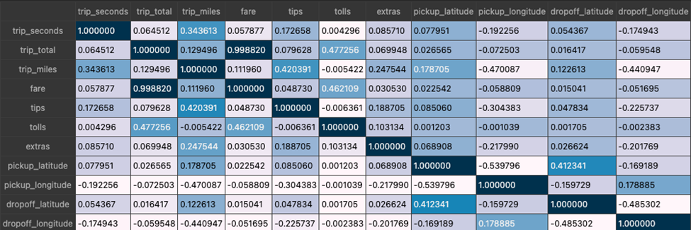
As a result of our data exploration, we found some interesting correlation patterns:

• - Strong correlations were identified between variables such as fare and trip_total, tolls,  and trip_total etc.
•  
• - Decisions were made to discard or keep variables based on correlation strength and relevance.
•  
•  

Missing Values:

• - A significant number of missing values were found in various columns. As a response to that, we decided to discard rows with missing values for selected features.
•  

Example Code Snippets

Check Missing Values:

SELECT count(*) FROM `gcp-ml-especialization-2024.spec_taxi_trips.taxi_trips`;

SELECT count(*) FROM `gcp-ml-especialization-2024.spec_taxi_trips.taxi_trips`

WHERE fare IS NULL;

Initial Raw Variables Key Findings and Data Transformation

During our analysis, we identified that some original variables in the dataset contained redundant information. Specifically, the dropoff_location variable, which held geolocation data as latitude/longitude pairs, duplicated information already present in the dropoff_latitude and dropoff_longitude variables. Consequently, we retained the latter two and discarded dropoff_location. These retained variables, along with pickup_latitude and pickup_longitude, will be used to create a new engineered feature called distance, representing the Euclidean distance between pickup and dropoff coordinates.

Example of dropoff_location Content

Snapshot of sample dropoff_location feature content

Similarly, the pickup_location variable was discarded from further analysis. Below is an example of its content:

Snapshot of sample pickup_location feature content

Key Findings on Trip Time-Related Information

Our dataset analysis revealed that only trip_start_timestamp and trip_end_timestamp variables contained time-related information in UTC. Duplicate timestamps across different trips were observed, prompting us to adopt a cross-sectional data analysis approach rather than a time-series/panel approach.

Using Pandas data frames in a Python notebook within Vertex Workbench, we created new time-related features such as minute, hour, day, day of the week, and month for each trip. These features were derived from trip_start_timestamp and trip_end_timestamp and will be detailed in the Feature Engineering section. Post-creation, the original timestamp variables were discarded.

Example of Time-Related Variables Content

Sample content of trip_start_timestamp and trip_end_timestamp

Distribution of Variables in the Dataset

We analyzed the distribution of variables using histograms and bar charts. Our findings indicate that most variables exhibit asymmetric distributions. For instance, the original target variable trip_seconds showed a right-hand skew before being transformed into trip_minutes.

Example of Trip Seconds Distribution

Trip_seconds sample distribution

Some variables, like dropoff_community_area, displayed multimodal distributions:

Barplot of dropoff_community_area

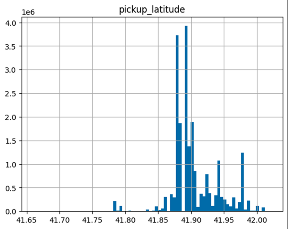
Others, such as pickup_latitude, showed a symmetric distribution:

Pickup latitude sample distribution

Data Transformation and Deep Learning Model Training

Given the plan to train a Deep Neural Network regressor for the trip_minutes target variable, no data transformations were implemented to alter feature distributions due to time constraints and the natural fit for deep learning models. However, other data transformations were implemented to expedite model training.

Data Type Changes

We changed the data type of trip_seconds from integer to float64, enabling the division by 60 to create the trip_minutes feature.

Min-Max Scaling

To enhance deep learning model training, we applied Min-Max Scaling to continuous variables using BigQuery SQL scripts. This scaling was implemented to improve data stability and performance.

Feature Engineering and Selection

Feature engineering steps were executed in a BigQuery script for performance optimization. The steps included:

1. Selecting desired fields and creating new features from timestamp variables.
   
2. Discarding null values.
3. Label encoding categorical variables.
4. Creating a new distance feature (Euclidean distance between pickup and dropoff coordinates).
5. Applying Min-Max scaling to continuous features.

The resulting dataset was stored in:

gcp-ml-especialization-2024.spec_taxi_trips.chicago_taxi_trips_final_dataset1.

By implementing these feature engineering and data preprocessing steps, we optimized the dataset for effective deep learning model training, validation, and testing.

Further Reduction of Variables in the Dataset for Model Training

Due to the substantial size of the datasets and the limitations of the available infrastructure for this demo, it was necessary to further reduce the dataset size. This required minimizing the number of features considered for Deep Learning Model training, and prioritizing the retention of most rows for each feature. Consequently, the following variables were discarded for model training, validation, and testing:

• Day_trip_start (redundant due to the day_of_the_week_trip_start variable)
• Hour_trip_end
• Day_trip_end
• Day_of_the_week_trip_end
• Fare
• Dropoff_latitude
• Dropoff_longitude
• Company_num
•  

The final datasets included these features:

• Hour_trip_start
• Day_of_week_trip_start
• Month_trip_start
• Trip_minutes (target variable)
• Trip_miles
• Pickup_latitude
• Pickup_longitude
• Distance

This resulted in a total of seven features and one target variable.

Preprocessing and the Data Pipeline

As depicted in the previous section, all data preprocessing was carried out using Big Query scripts. The final tables used in model training, validation and test were made available by the Big Query functionality/API that is callable from within the Jupyter notebooks, to read Big Query tables as Pandas dataframes from within Vertex Workbench for model training validation and testing.

For the deployed model, the model endpoint is able to receive requests in JSON formats, in .csv files sitting in Cloud Storage or reading from Big Query tables, both for batch predictions as well as for online predictions.

We now present the feature engineering Big Query script in the code snippet below:

WITH temp1 AS (

   SELECT

       --taxi_id,

       --trip_start_timestamp,

       --trip_end_timestamp,

       EXTRACT(MINUTE FROM trip_start_timestamp AT TIME ZONE "UTC") as minute_trip_start,

       EXTRACT(HOUR FROM trip_start_timestamp AT TIME ZONE "UTC") as hour_trip_start,

       EXTRACT(DAY FROM trip_start_timestamp AT TIME ZONE "UTC") as day_trip_start,

       EXTRACT(DAYOFWEEK FROM trip_start_timestamp AT TIME ZONE "UTC") as day_of_week_trip_start,

       EXTRACT(MONTH FROM trip_start_timestamp AT TIME ZONE "UTC") as month_trip_start,

       --EXTRACT(YEAR FROM trip_start_timestamp AT TIME ZONE "UTC") as year_trip_start,

       EXTRACT(MINUTE FROM trip_end_timestamp AT TIME ZONE "UTC") as minute_trip_end,

       EXTRACT(HOUR FROM trip_end_timestamp AT TIME ZONE "UTC") as hour_trip_end,

       EXTRACT(DAY FROM trip_end_timestamp AT TIME ZONE "UTC") as day_trip_end,

       EXTRACT(DAYOFWEEK FROM trip_end_timestamp AT TIME ZONE "UTC") as day_of_week_trip_end,

       EXTRACT(MONTH FROM trip_end_timestamp AT TIME ZONE "UTC") as month_trip_end,

      -- EXTRACT(YEAR FROM trip_end_timestamp AT TIME ZONE "UTC") as year_trip_end,

       CAST(trip_seconds AS float64)/60  AS trip_minutes,

       trip_miles,

       --pickup_census_tract,

       --dropoff_census_tract,

       pickup_community_area,

       dropoff_community_area,

       fare,  

       tips,

       --tolls,

       extras,

       trip_total,

       payment_type,

       company,

       ROUND(pickup_latitude,3) as pickup_latitude,

       ROUND(pickup_longitude,3) as pickup_longitude,

       --pickup_location,

       ROUND(dropoff_latitude,3) as dropoff_latitude,

       ROUND(dropoff_longitude,3) as dropoff_longitude,

       --dropoff_location

       ST_DISTANCE(ST_GEOGPOINT(pickup_longitude,pickup_latitude),ST_GEOGPOINT(dropoff_longitude,dropoff_latitude)) as distance

       FROM `gcp-ml-especialization-2024.spec_taxi_trips.taxi_trips`

       --WHERE trip_start_timestamp ='2013-01-01T00:00:00.000Z'

)

-- Eliminating NULL VALUES in all fields

, temp2 as (

   SELECT * FROM temp1

   WHERE

   minute_trip_start IS NOT NULL AND

   hour_trip_start IS NOT NULL AND

   day_trip_start IS NOT NULL AND

   day_of_week_trip_start IS NOT NULL AND

   month_trip_start IS NOT NULL AND

   minute_trip_end IS NOT NULL AND

   hour_trip_end IS NOT NULL AND

   day_trip_end IS NOT NULL AND

   day_of_week_trip_end IS NOT NULL AND

   month_trip_end IS NOT NULL AND

   trip_minutes IS NOT NULL AND

   trip_miles IS NOT NULL AND

   pickup_community_area IS NOT NULL AND

   dropoff_community_area IS NOT NULL AND

  fare IS NOT NULL AND

  --tolls IS NOT NULL AND

  extras IS NOT NULL AND

  trip_total IS NOT NULL AND

  payment_type IS NOT NULL AND

  company IS NOT NULL AND

  pickup_latitude IS NOT NULL AND

  pickup_longitude IS NOT NULL AND

  dropoff_latitude IS NOT NULL AND

  dropoff_longitude IS NOT NULL AND

  distance IS NOT NULL

)

-- Label encoding of company categorical variable

, temp3 as (

   SELECT

   company,

   DENSE_RANK() OVER (ORDER BY company ASC) AS company_num

   FROM

   (

       SELECT DISTINCT company FROM temp2

   )

)

, temp4 as (

   SELECT * FROM temp2

   LEFT JOIN temp3 USING (company)

)

-- Label encoding of payment_type categorical variable

, temp5 as (

   SELECT

   payment_type,

   DENSE_RANK() OVER (ORDER BY payment_type ASC) AS payment_type_num

   FROM

   (

       SELECT DISTINCT payment_type FROM temp4

   )

)

, temp6 as (

   SELECT * FROM temp4

   LEFT JOIN temp5 USING (payment_type)

)

-------

, temp7 as (

SELECT

       --taxi_id,

       --trip_start_timestamp,

       --trip_end_timestamp,

       payment_type,

       company,

       minute_trip_start,

       hour_trip_start,

       day_trip_start,

       day_of_week_trip_start,

       month_trip_start,

       --year_trip_start,

       minute_trip_end,

       hour_trip_end,

       day_trip_end,

       day_of_week_trip_end,

       month_trip_end,

      -- year_trip_end,

       ML.MIN_MAX_SCALER(trip_minutes) OVER() as trip_minutes,

       ML.MIN_MAX_SCALER(trip_miles) OVER() as trip_miles,

       --pickup_census_tract,

       --dropoff_census_tract,

       pickup_community_area,

       dropoff_community_area,

       ML.MIN_MAX_SCALER(fare) OVER() as fare,  

       ML.MIN_MAX_SCALER(tips) OVER() as tips,

       --tolls,

       ML.MIN_MAX_SCALER(extras) OVER() as extras,

       ML.MIN_MAX_SCALER(trip_total) OVER() as trip_total,

       ML.MIN_MAX_SCALER(pickup_latitude) OVER() as pickup_latitude,

       ML.MIN_MAX_SCALER(pickup_longitude) OVER() as pickup_longitude,

       --pickup_location,

       ML.MIN_MAX_SCALER(dropoff_latitude) OVER() as dropoff_latitude,

       ML.MIN_MAX_SCALER(dropoff_longitude) OVER() as dropoff_longitude,

       --dropoff_location,

       ML.MIN_MAX_SCALER(distance) OVER() as distance,

       company_num,

       payment_type_num

       FROM temp6

)

-------

, final1 as (

   SELECT * FROM temp7

)

select * from final1

Below we present a CODE SNIPPET for reading Big Query Tables in Vertex AI as Pandas dataframes:

Machine Learning  Model Design and Selection

The machine learning models considered for this demo, are deep learning neural networks models.

The model selection criteria used model selection was model performance in the validation set, according to the performance metrics adopted (MSE, r2 coefficient and explained variance).  The final chosen model was the one with highest explained variance and r2 and the same time,  did not present very high MSE.

Machine Learning model training and development

Dataset Sampling for Model Training, Validation, and Test

The dataset was split into training, validation, and test sets using the trip_start_timestamp field. Random sampling was unnecessary. Instead, we have splitted original dataset using the timestamp variable trip_start_timestamp in the following manner:

- Train dataset was formed with observations ranging from trip_start_timestamp ranging from '2013-01-01 00:00:00 UTC' AND '2018-01-21 23:45:00 UTC',

-       Validation dataset was formed with observations ranging from trip_start_timestamp ranging from '2018-01-21 23:45:01 UTC' AND '2018-10-24 23:45:00 UTC',

-       Test dataset was formed with observations ranging from trip_start_timestamp greater than '2018-10-24 23:45:00 UTC' .

Train, Validation, and Test Splits were accomplished in such a way that The dataset was split into train (70% of the data), validation (20% of the data), and test (10%of the data) sets based on trip_start_timestamp field.

The following queries were accomplished in Big Query to create these datasets:

Train Dataset Creation

SELECT *

FROM `gcp-ml-especialization-2024.spec_taxi_trips.chicago_taxi_trips_final_dataset1`

WHERE trip_start_timestamp BETWEEN '2013-01-01 00:00:00 UTC' AND '2018-01-21 23:45:00 UTC';

Validation Dataset Creation

SELECT *

FROM `gcp-ml-especialization-2024.spec_taxi_trips.chicago_taxi_trips_final_dataset1`

WHERE trip_start_timestamp BETWEEN '2018-01-21 23:45:01 UTC' AND '2018-10-24 23:45:00 UTC';

Test Dataset Creation

SELECT *

FROM `gcp-ml-especialization-2024.spec_taxi_trips.chicago_taxi_trips_final_dataset1`

WHERE trip_start_timestamp > '2018-10-24 23:45:00 UTC';

Proposed Machine Learning Model

We chose deep neural network regression models for predicting taxi trip durations in Chicago. No special components (e.g., convolutional layers) were needed in the deep learning models architecture. Rectified Linear Activation functions were adopted in all layers for their beneficial properties in deep architectures. The Adam optimization algorithm was selected to address common issues like gradient vanishing in deep neural networks.

Framework Used

The Keras framework (with TensorFlow backend) was used, specifically version 2.12.0, due to Google Cloud's constraints for model registry and deployment. Keras was chosen for its abstraction over TensorFlow, simplifying model specification and training.

Deep Neural Network Architecture Choice

The final architecture was influenced by several factors:

• Available infrastructure resources (memory and computation time)
• Size of the training dataset
• Time constraints for development (data exploration, feature engineering, model training, evaluation, testing, and deployment)
• Testing of the deployed model with batch predictions using Google Cloud solutions

After evaluating different architectures, the final neural network included:

• Input layer: Densely connected with ReLU activation, seven nodes
• Second layer: Densely connected with ReLU activation, five nodes
• Third layer: Densely connected with ReLU activation, three nodes
• Fourth layer: Densely connected with ReLU activation, two nodes
• Output layer: One node for regression prediction
•  

Hyperparameter tuning, performance optimization and Training Configuration

Regarding hyperparameter tuning, the main hyperparameter considered was the learning rate used for the training process. The model performance optimization was aimed to increasing r2 and explained variance  while reducing MSE.

 Three different deep learning models were trained, each one considering a different architecture and a given learning rate. The first trained model used a learning rate of 0.8, the second one a learning rate of 0.08 and the third (chosen final) model a learning rate of 0.01. So that hyperparameter tuning was done along these three training sessions.

The final training session ran for 10 epochs with the following additional parameters:

• Beta_1: 0.9
• Beta_2: 0.999
• Epsilon: None
• Decay: 0.0
• Amsgrad: False

Model training

All the models trained in this demo used the Adam optimization algorithm. As explained, each model used a different set of hyperparameters (including the learning rate, and the number of epochs) for training, in the previous section. All training sessions were conducted using the same training dataset (chicago_taxi_trips_final_dataset_train table).

Adherence to Google’s Machine Learning Best Practices

Regarding adherence to Google`s Machine learning Best Practices, several best practices were followed in this development, such as:

• Maximization of  model`s predictive precision with hyperparameters adjustments.
• Preparation of models artifacts to be available in Cloud Storage: this was accomplished in Demo 1 where models`s artifacts were made available in TensofFlow format (saved_model.pb files) .
• Specification of the number of cores and machine specifications for each project: we have defined appropriate machines (in terms of number of cores, memory and even GPU`s to be used in each Demo based on previous experience).

Machine Learning Model Evaluation and Performance Assessment

The MSE metric was selected to assess model performance on training, validation, and test sets, as it emphasizes large errors and is a standard metric in academia and industry. Other metrics used included Mean Absolute Error (MAE), determination coefficient (R2), and Root Mean Squared Error (RMSE).

Bias/ Variance tradeoff

The model bias/ variance tradeoff were determined by analyzing the models performance metrics conjointly in the validation dataset.

The best model was considered the one with highest explained variance and r2 and that, at the same time did not presented very high MSE.

Final Obtained Results

The final trained model achieved the following results on the validation set:

Figure: Final Regression Model Performance on Validation Set

The deep learning regression model explained 27.3% of the variance in the validation set, which is considered suboptimal.

On the test set, the final regression model obtained the following results:

Figure: Final Regression Model Performance on Test Set

The model explained 23.98% of the variance in the test set, also considered suboptimal.

Given the constraints faced during development, these were the best achievable results. However, the main purpose of this use case was to demonstrate a complete workflow implementation of a machine learning solution using Google Cloud. This objective was successfully fulfilled.

Final Considerations and Recommendations for Future Developments

Suggested Actions for Improvement

To substantially improve the model's performance, consider the following next steps:

1.     Feature Selection: Due to constraints, the training sessions used the same feature set, which may not have been optimal. Implement a feature selection algorithm, such as Mutual Information, on a dataset sample to better guide feature selection for future models. This should yield a more significant set of features for neural network models.
2.     Neural Network Architectures: The development tested a limited number of neural network architectures. Future work should explore a broader range of architectures, including more layers and varying numbers of neurons in each layer.
3.     Hyperparameter Optimization: Experiment with different combinations of hyperparameters, as they are crucial for deep learning model performance.

The main objective of this development was to present a complete workflow for developing a machine learning model to meet specific business needs using Google Cloud. This project provided a detailed description of all steps involved (from data exploration to model deployment) while adhering to Google Machine Learning Best Practices. Recommendations for future developments were also provided.