
Have you ever wondered how to convert a prediction problem into a new format so that you can solve it using available strong forecasting engines? In Part I of this tutorial, I will discuss how to solve one of the most challenging forecasting problems--the next state forecasting trend of electricity consumption--by using a Deep Convolutional Neural Network (DCNN) to process a series of load data that’s been converted into images.
This solution enables a possible testing set accuracy of 88%, which is impressive for this type of application. For the programming component, we’ll use Python and Tensorflow.
Introduction to CNNs
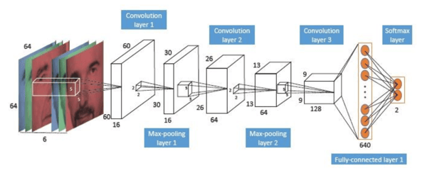
Before beginning this tutorial, let’s review some fundamentals about Deep Neural Networks. Deep Neural Networks (DNNs) learning is part of a broader family of machine learning methods based on learning data representations as opposed to task-specific algorithms. Convolutional Neural Networks (CNNs), which we’re using to solve today’s problem, are a subset of DNNs. Convolutional networks were inspired by biological processes in that the connectivity pattern between neurons resembles the organization of the animal visual cortex, where individual cortical neurons respond to stimuli only in a restricted region of the visual field known as the receptive field. DCNNs, however, are typically organized into alternating convolutional and max-pooling neural network layers followed by a number of dense, fully-connected layers, a structure that was introduced by Krizhevsky et al. An example of DCNN topology can be seen in the following image. (For a simple and detailed explanation of DCCNs, click here.)
The structure of DCNNs makes them very suitable for image classification and automatic speech recognition. In this tutorial, we will examine how to use DCNNs to solve an electricity consumption prediction.
A New Application for DCNNs
So far, DCNNs have been primarily used in computer vision applications, such as facial recognition, image classification, action recognition, and natural language processing (speech recognition, text classification, etc.). In this blog, however, I am going to show that DCNNs can also be used in the completely unrelated field of electricity consumption forecasting. We’ll also discuss how to prepare data to feed into a DCNN, which is a process that goes almost entirely unaddressed in existing Tensorflow tutorials. Lastly, I will also discuss details about the models, along with their related technical programming parts.
Why Accurate Forecasting for Electrical Consumption is Critical
Short-term load forecasting is vital for all energy supply companies. If demand is underestimated, consumers’ needs are unmet, yet if it is overestimated, electrical energy will be wasted since it cannot be stored. For enterprise companies, every percentage point gained in accurate forecasting can translate to as much as $15,000 saved daily, making accurate forecasting critical. Consumer demand for electricity, however, is always in flux and is influenced by a number of complex factors for which statistical forecasting models must account. We will use a DCNN today because such models are designed to automatically extract features from data.
Data
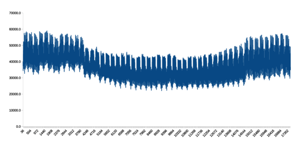
For the purposes of this blog, we are using a series containing 17,520 items of half-hourly electricity consumption records for one full year of data from a big power supply company. As seen below, the time series is very complicated and contains several hidden seasonality patterns that our DCNN can easily capture and use to produce a relatively accurate prediction. As with any DNN model, our DCNN requires plenty of training data to produce an accurate result, so our time series sample below is sufficient to build a good forecasting model. You can download data here.
Methodology
Because DCNNs are designed to interpret data in the form of images, we will convert our half-hourly load data into gray-scale images with their associated classes. The classes/labels that we are going to predict are 1 if the consumption of the next half hour of electricity compared with the current state is going up or 0 if it is going down. Our methodology, then, involves converting half-hourly load data into several images that can be used to predict the trend in sequential electricity consumption.
Data Preprocessing
Before using our DCNN for time series forecasting, we have to convert equal chunks of time series into images. To show how this works, we’ll use this small and extremely simplified time series as an example:
[23, 45, 31, 95, 81, 52, 83, 56]
Suppose that the width and height of the images we are going to make are both 4. (Later, in our real case, the width and height will both be 32.)
Step 1: From left to right, select 4 numbers and create successive vectors with four rows of windows until we reach the end of the 4 x 4 series:
[23, 45, 31, 95]
[45, 31, 95, 81]
[31, 95, 81, 52]
[95, 81, 52, 83]
Step 2: Next, we need to produce a label for each window. If the last value in a vector is less than the last value in the next vector, then we will assign 1 to that vector label. If it is greater, we assign 0. This gives us:
[23, 45, 31, 95] 0 (because 81 is less than 95)
[45, 31, 95, 81] 0 (because 52 is less than 81)
[31, 95, 81, 52] 1 (because 83 is greater than 52)
[95, 81, 52, 83] 0 (because 56 is less than 83
We assign values of 0 and 1 to help us predict whether the energy consumption of the next state of time will increase or decrease from the current state. This helps us build a training set.
Step 3: For each vector, keep and put the position of the members of the equivalent sorted vector correspond to other members of the main vector, in a new array, so the following is the output,
[0, 2, 1, 3] 0 (position of 23 is in 0th position, 45 is in 2th, for 31 it is 1th, etc.)
[1, 0, 3, 2] 0
[0, 3, 2, 1] 1
[3, 1, 0, 2] 0
Step 4: Finally, we now have enough information to build our gray-scale images. For each member of each vector obtained from a former step, add a corresponding vector. By using one hot encoding techniques, we can create an equivalent matrix that can be interpreted as gray-scale images as follows
1, 0, 0, 0
0, 0, 1, 0 0
0, 1, 0, 0
0, 0, 0, 1
0, 1, 0, 0
1, 0, 0, 0 0
0, 0, 0, 1
0, 0, 1, 0
1, 0, 0, 0
0, 0, 0, 1 1
0, 0, 1, 0
0, 1, 0, 0
0, 0, 0, 1
0, 1, 0, 0 0
1, 0, 0, 0
0, 0, 1, 0
Next Steps
By following these last steps, we can establish our gray-scale images and their corresponding labels. In our application, however, the width and height of images are both 32, so each image is going to be a numpy array of 32 x 32 dimensions. We will feed these images into a DCNN to train our classification model in order to build a prediction model which can predict the trend in the next half-hour consumption of electricity. In our next blog, we will develop a Python class to employ the data produced above in conjunction with developing a Tensorflow model for deploying DCNNs.
Conclusion
In this tutorial, we explained how to build a forecasting model for time series analysis by using DCNNs. To employ a DCNN, we first need to convert our time series into images. To do so, we showed a step-by-step process of preparing data in text. In our next blogs, we will use Python and Tensorflow to finish solving the problem. The codes related to this problem will be discussed as well.


