
We consider optimization every day of our lives. We always want to take the route that will get us to work the fastest, accomplish as many tasks as possible on time based on priority, and so on. Optimization means finding the solution (or solutions) for a problem that produces a result that cannot be further improved. Today, we'll introduce multiple objective optimization.
Numerical Optimization
We refer to numerical optimization when we talk about improving the result of a mathematical problem. This is used in engineering, biology, economics, and aerospace design, to name a few. Think about the challenge of modelling the wing of an airplane to minimize resistance and maximize lift. An ideal solution would probably cheapen costs for both the airline and the customers.
While this article does not intend to solve such a complex problem (entire theses have been devoted to solving airfoil design), it tries to give a brief introduction to numerical optimization without going too much into the technical side of things. In addition, while we use Swift to generate the example functions, no previous knowledge of Swift is required to understand the concepts we'll cover.
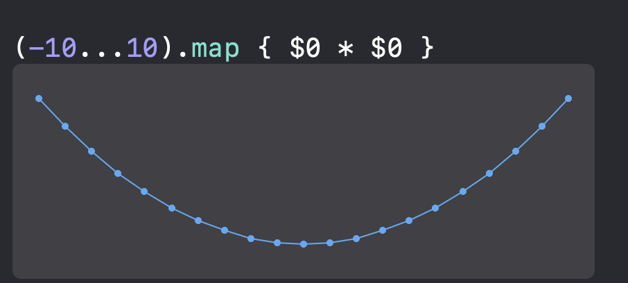
Let’s start with a basic optimization example. Say we were given the problem of finding the minimum of the function x^2 (or x times x); we could say that the best solution would be when x = 0, since 0^2 = 0. We know that there is no other solution (for real numbers) that would yield a number less than 0.
We can easily see this when we plot this function:
In Single Objective Optimization, we would search for the best solution for only one problem at a time. But what happens if we want to find the best solution for more than one problem? We then enter in a field called Multiple Objective Optimization, or MOO for short.
Multiple Objective Optimization
In MOO, we usually want to either minimize or maximize multiple functions simultaneously. However, these functions are often in conflict with one another. An improved solution for one function often means a worse solution for another function. In such cases, we are left with a group of optimal solutions. This group, or set of solutions, is referred to as the Pareto set, while the result of evaluating the Pareto set in the function is called the Pareto front. (I won't go into details regarding the mathematical definition of the Pareto set, since this is out of scope for the purpose of this post. The original article can be found here).
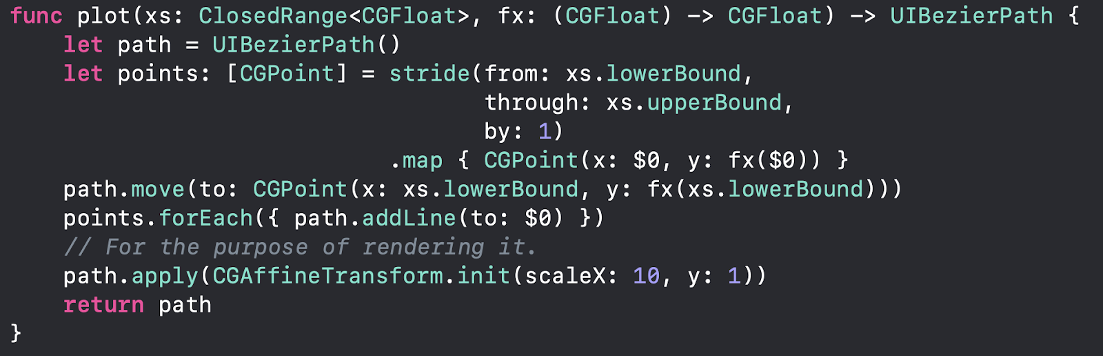
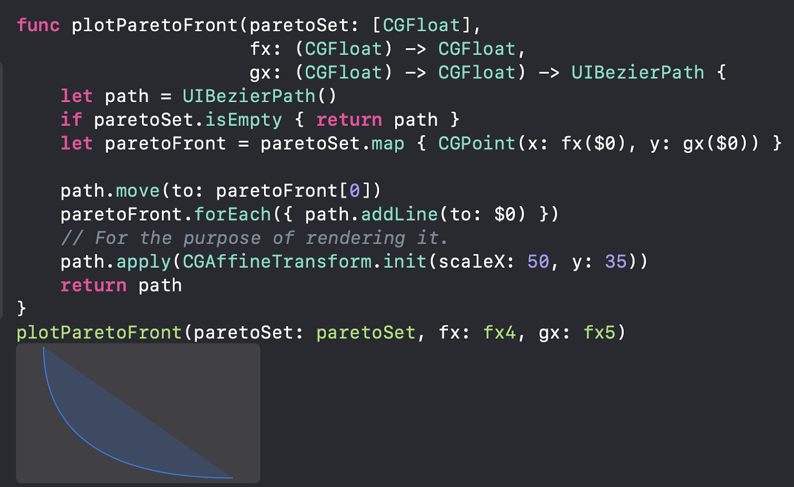
To illustrate MOO, I've created a small function that takes in a range of values and a given function. We then use this range to evaluate the given function and create a set of CGPoints to add into our plot, as shown below:
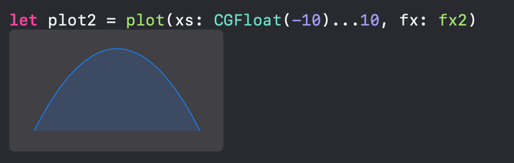
Now that we have our plotting function, we can illustrate a simple example. Consider the following two functions:
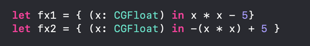
The first function is a simple quadratic function.
The second function is also quadratic. The only difference is that we are flipping the y-values and shifting the result up by a fixed amount.
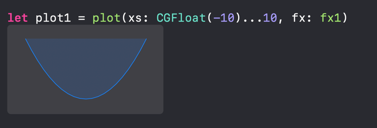
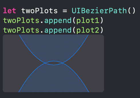
If we were to plot our two functions, we'd see something like the image below. Notice the intersection between the two functions. Here, the functions are in conflict since decreasing our first function increases the value of the second function.
There are a number of approaches to obtain the Pareto set for MOO problems, including scalarization techniques, line search methods, and evolutionary algorithms. Due to the scope of this post, I’ll only show an example of a scalarization method. This method will serve as an introductory point for the subject, since more advanced methods involve evolutionary algorithms and a deeper understanding of numerical optimization.
Scalarization Methods
These methods aim to reduce the MOO problem into a single objective one and then find the solution to the problem.
Weighted Sum Method
The Weighted Sum Method was proposed by Lotfi Zadeh. The idea behind this method is to associate a weight, or scalar value, to each function and then combine the functions into one. So if we have the two functions f(x) and g(x), we could reduce this problem to:
h(x) = w₁f(x) + w₂g(x), where w₁ and w₂ are scalar values, and where w₁+w₂ = 1.
Going back to our original problem, we could set these scalar values to, say, 0.5 each. This means that we value both functions equally, and thus, the resulting solution would be:
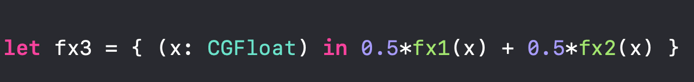
So if we wanted to get the smallest possible value on this function, we'd have:
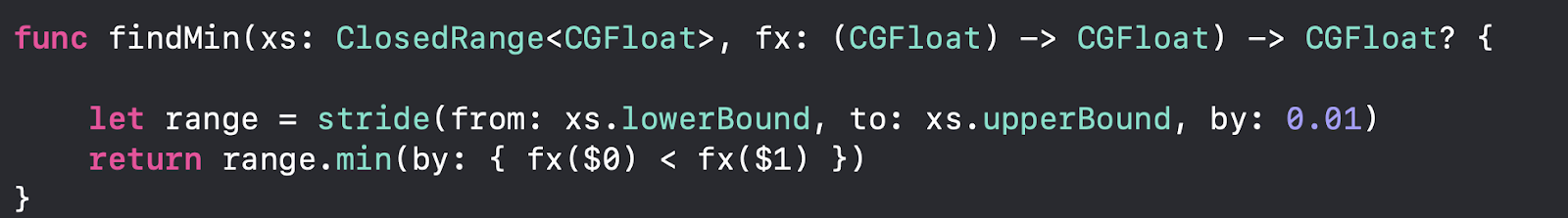
Since we merged both functions into one, what we get is a single optimization problem, which means a single optimal solution for the given set of weights. This is, in fact, the main drawback of scalarization methods. We can, however, have an even distribution of weights, which would result in a set of optimal solutions, but that still doesn't guarantee an even distribution of points in the Pareto front.
Let's try a different example now. Suppose we have the following functions:

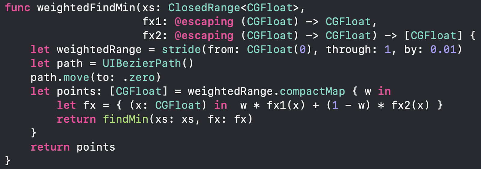
Using the Weighted Sum method, we can obtain the Pareto set using the given range.

We can then use this function to plot the Pareto front, which shows the set of optimal solutions when we change the value of the weights.
We have to take into account the following things, though:
- We haven't covered the entire range of possible weight values, which means that we haven't explored the entirety of the set of solutions.
- More importantly, we didn't fully test the range of x values. In this particular example, it's of little consequence, but for other MOO problems, we could miss parts of the Pareto front entirely.
Conclusion
As you can see, MOO is a complex field, and what's shown here is just the tip of it. Over the course of the years, new techniques and algorithms have been developed to try to solve MOO problems while reducing the computational effort and time it takes to analyze them.
We’ll always see numerical optimization in our everyday lives, even if we don’t realize it. But now, every time you see a SpaceX rocket launch, you can think to yourself: someone had to solve a MOO problem by minimizing the fuel spent while maximizing the lift. I hope you enjoyed this article, even if it was not as Swift-y as you might have expected!


